球面高斯函数04——球面高斯光源的镜面高光

上篇文章中，讨论了使用漫反射BRDF时如何计算球面高斯光源的分布。下面可以讨论如何计算与视角有关的更复杂的BRDF，这样就可以得到高光的分布。本文会介绍如何逼近基于微表面的镜面反射BRDF对球面高斯光源的反应情况，并且会介绍各向异性球面高斯的概念。

本系列的其他文章可以点击下方链接跳转。

• Part1-光照贴图简史
• Part2-球面高斯函数101
• Part3-球面高斯光源的漫射照明
• Part4-球面高斯光源的镜面高光
• Part5-用球面高斯函数近似辐射率和辐射度

微平面镜面反射

迪士尼提出的基于物理的渲染公式是当下实时渲染领域比较流行，应用最广的。其中基于微平面的镜面反射BRDF如下：

$$\begin{align} f(i,o)=\frac{F(o,h)G(i,o,h)D(h)}{4(n\cdot{i})(n\cdot{o})} \nonumber \end{align}$$

D项通常称为法线分布函数(Normal Distribution Function, NDF)，描述微面元法线分布的概率，即正确朝向的法线的浓度。可以在粗糙度上做参数化，描述微平面的凹凸程度。低粗糙度会产生锐利清晰的镜面反射和狭窄细长的镜面波瓣；高粗糙度会产生更宽的镜面波瓣。大多数的现代游戏(包括教团:1886)的D项都用的GGX(Trowbridge-Reitz)分布。下面两图都使用的GGX分布，分别使用0.5的粗糙度和0.1的粗糙度；X轴是表面法线和半角向量的夹角。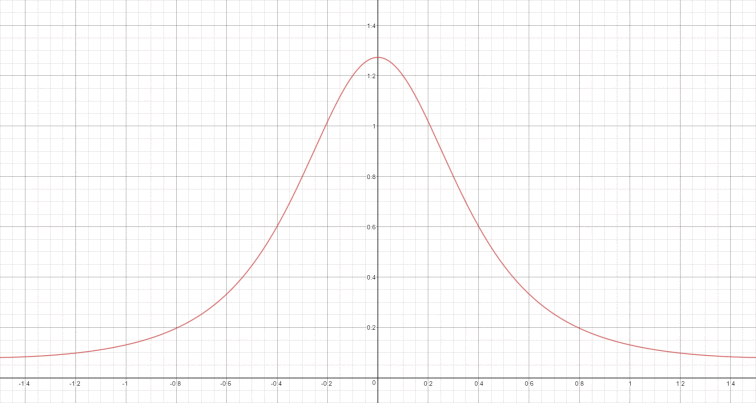

G项是几何函数(Geometry Function)，也被称为掩蔽阴影函数(Masking-Shadow Function)。描述微平面自成阴影的属性，即微面元法线与面法线一致并未被遮蔽的表面点的百分比。下图使用的是Smith-GGX函数作为G项的曲线，粗糙度为0.25，法线与视线夹角为0。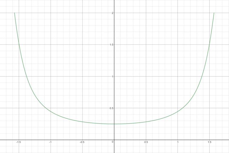

F项是菲涅尔方程(Fresnel Equation)，描述不同的表面角下表面所反射的光线所占的比率。从F0到F90，反射强度逐渐增加。使用Schilick近似表示菲涅尔项的曲线如下，F0=0.04：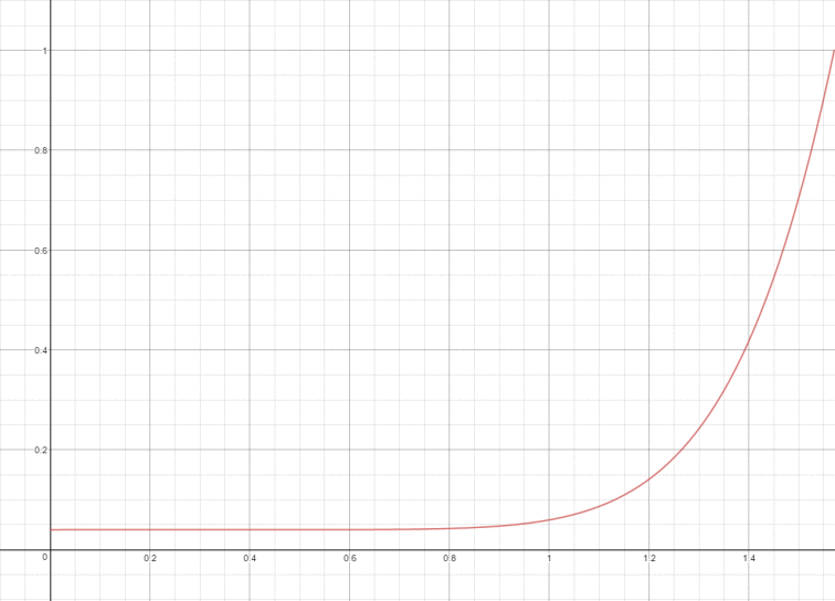

球面高斯光源的镜面反射

沿用迪士尼的镜面反射BRDF，为了与精确光源以及IBL探针正常交互。但会按照球面高斯光源对其拓展：

$$\begin{align} L_o(0,x) = \int_{\Omega}\frac{F(o,h)G(i,o,h)D(h)G_l(i;\mu,\lambda,a)cos(\theta_i)d\Omega}{4cos(\theta_i)cos(\theta_o)} \nonumber \end{align}$$ $$\begin{align} L_o(0,x) = \int_{\Omega}\frac{F(o,h)G(i,o,h)D(h)ae^{\lambda(\mu\cdot{i}-1)}d\Omega}{4cos(\theta_o)} \nonumber \end{align}$$

与漫反射不同，现在积分中有多个项与视角有关。那么需要做一些激进的优化得到期望的结果。

D项

D项是镜面反射BRDF中最重要的项。该分布决定了镜面高光整体的形状和强度，如果回看GGX曲线，其走势类似于高斯曲线，但不完全匹配。用单个球面高斯是不能实现紧凑高光和长拖尾的的特征。可以把多个高斯相加去逼近，但本文会用简单的单波瓣去近似。《All-Frequency Rendering of Dynamic, Spatially-Varying Reflectance》中提出过一种逼近Cook-Torrance D项的一个简单公式：

$$\begin{align} D(h) = e^{-(arccos(h\cdot n)/m)^{2}} \approx G(h;n,\frac{2}{m^2},l) \nonumber \end{align}$$

但该高斯模型的峰值并不会随着粗糙度变化而变化，好在有简单的分析公式可以计算球面高斯的积分，因此可以将整个积分的幅度值设置为1，这样一个归一化的D项就是：

$$\begin{align} D_{SG}(h) = G(h;n,\frac{2}{m^2},\frac{1}{\pi m^2}) \nonumber \end{align}$$

SG DistributionTermSG(in float3 direction, in float roughness)
{
    SG distribution;
    distribution.Axis = direction;
    float m2 = roughness * roughness;
    distribution.Sharpness = 2 / m2;
    distribution.Amplitude = 1.0f / (Pi * m2);
 
    return distribution;
}

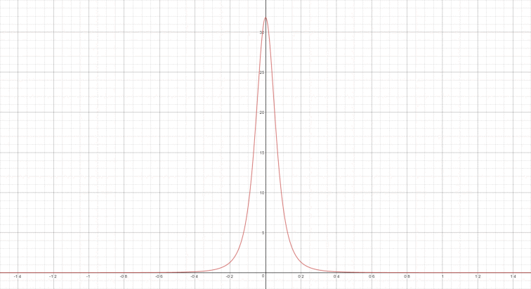
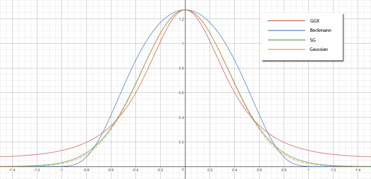
下方的图标显示了当前的近似方式与GGX的差距，上图粗糙度为0.25，下图粗糙度为0.5：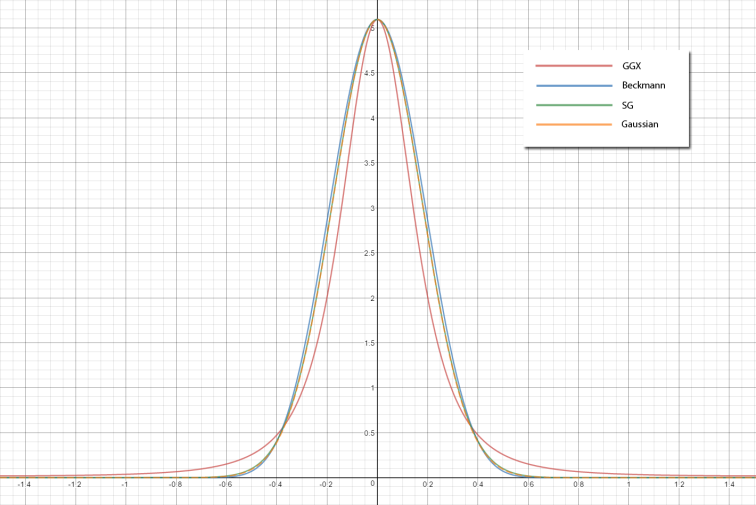

域之间的扭曲

现在有了球面高斯格式的法线分布函数，但却无法使用。因为我们是在半角向量中定义的分布函数，球面高斯的轴是指向面法线方向的，而且我们使用半角向量作为采样方向。如果要使用球面高斯积运算来获取球面高斯光源下的分布，必须保证分布波瓣和光源在同一个域的。换言之，分布的中心是随着观察角度变化的，因为半角向量会随着观察方向改变。

为了确保分布波瓣在正确的域中，需要对其扭曲来对齐观察方向的BRDF切片。对于微平面的镜面反射BRDF来说，波瓣是围绕视线反射方向大致居中的。下方图表就是GGX的波瓣，蓝线为观察方向，绿线是面法线方向，粉线是视线反射方向。上图视角为0度，下图视角为45度。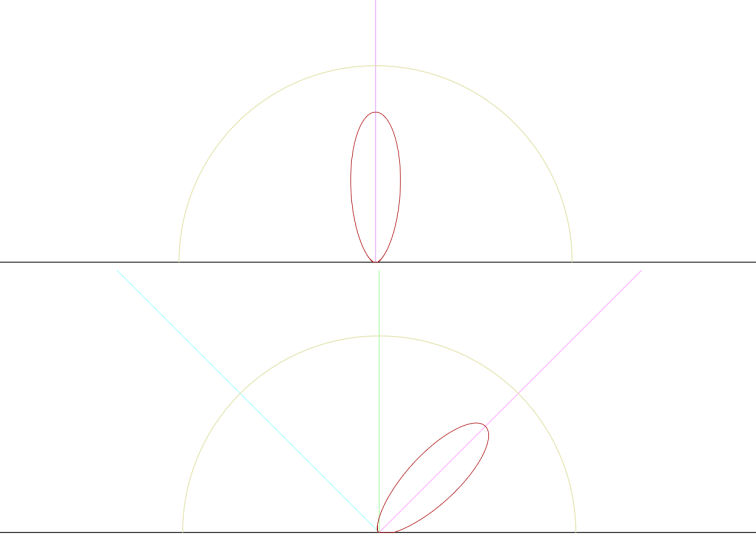

《All-Frequency Rendering of Dynamic, Spatially-Varying Reflectance》中提供了一个简单的扭曲算子，可以是分布波瓣围绕视线反射方向旋转，并且根据原始波瓣中心的差异差异调整锐度。

$$\begin{align} \mu_w = 2(o\cdot \mu_d)\mu_d - o \nonumber \end{align}$$ $$\begin{align} \lambda_w = \frac{\lambda_d}{4|\mu_d\cdot o|} \nonumber \end{align}$$ $$\begin{align} a_w = a_d \nonumber \end{align}$$

SG WarpDistributionSG(in SG ndf, in float3 view)
{
    SG warp;
 
    warp.Axis = reflect(-view, ndf.Axis);
    warp.Amplitude = ndf.Amplitude;
    warp.Sharpness = ndf.Sharpness;
    warp.Sharpness /= (4.0f * max(dot(ndf.Axis, view), 0.0001f));
 
    return warp;
}

现在对比一下扭曲后的球面高斯分布项与GGX分布的差异，红色是GGX分布，绿色是球面高斯分布：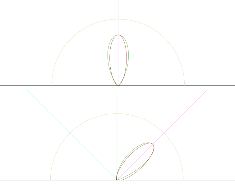

形状稍有偏离，但扭曲后的波瓣出现在了正确的位置上。

剩余项的近似

剩余的G项和F项和高斯分布相差甚远，所以不能用球面高斯去近似。《All-Frequency Rendering of Dynamic, Spatially-Varying Reflectance》中针对此问题做了一些假设来回避此问题，即这些项的值在整个BRDF波瓣中保持不变，这样就可以把它们从积分中提出来，并仅针对BRDF波瓣的轴向进行评估。这使得BRDF在掠射角仍然有效果。但是随着粗糙度增加，G项和F项会离波瓣中心越远，BRDF波瓣会变宽，误差会变得明显。

$$\begin{align} f_{sg}(i,o) = \frac{F(o,h_w)G(\mu_w,o,h_w)\frac{1}{\pi m^2}e^{\lambda_w(\mu_w \cdot i -1)}}{4(n\cdot \mu_w)(n \cdot o)} \nonumber \end{align}$$ $$\begin{align} h_w = \frac{o+\mu_w}{||o+\mu_w||} \nonumber \end{align}$$

最后是半球积分中与BRDF相乘的余弦项。《All-Frequency Rendering of Dynamic, Spatially-Varying Reflectance》中建议使用球面高斯乘积来得到一个球面高斯，该球面高斯表示球面高斯分布项与钳制余弦波的近似球面高斯相乘的结果。为了降低开销，采用G项与F项的方式，只会在BRDF波瓣的轴的方向评估余弦项。代码如下：

float GGX_V1(in float m2, in float nDotX)
{
    return 1.0f / (nDotX + sqrt(m2 + (1 - m2) * nDotX * nDotX));
}
 
float3 SpecularTermSGWarp(in SG light, in float3 normal,
                          in float roughness, in float3 view,
                          in float3 specAlbedo)
{
    // Create an SG that approximates the NDF.
    SG ndf = DistributionTermSG(normal, roughness);
 
    // Warp the distribution so that our lobe is in the same
    // domain as the lighting lobe
    SG warpedNDF = WarpDistributionSG(ndf, view);
 
     // Convolve the NDF with the SG light
    float3 output = SGInnerProduct(warpedNDF, light);
 
    // Parameters needed for the visibility
    float3 warpDir = warpedNDF.Axis;
    float m2 = roughness * roughness;
    float nDotL = saturate(dot(normal, warpDir));
    float nDotV = saturate(dot(normal, view));
    float3 h = normalize(warpedNDF.Axis + view);
 
    // Visibility term evaluated at the center of
    // our warped BRDF lobe
    output *= GGX_V1(m2, nDotL) * GGX_V1(m2, nDotV);
 
    // Fresnel evaluated at the center of our warped BRDF lobe
    float powTerm = pow((1.0f - saturate(dot(warpDir, h))), 5);
    output *= specAlbedo + (1.0f - specAlbedo) * powTerm;
 
    // Cosine term evaluated at the center of the BRDF lobe
    output *= nDotL;
 
    return max(output, 0.0f);
}

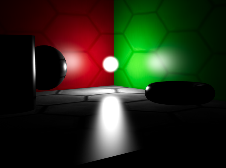
下图是使用球面高斯光源照亮的场景，并使用上文中所有的镜面反射近似方式后的结果，场景的粗糙度为0.128。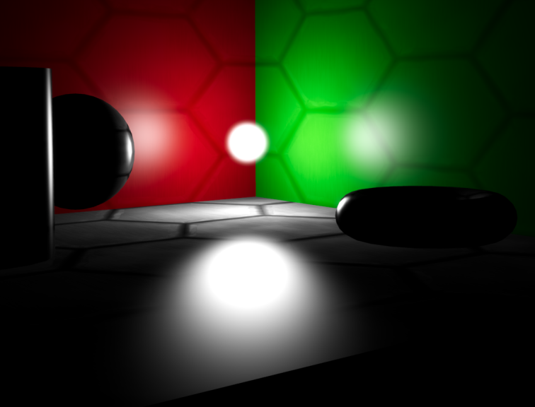

各向异性

上图中地板的高光又宽又圆，正常的掠射角观察的高光应该会延伸到较远的地方。所以需要重新检查一下D项。下方的3D示意图分别是观察角度较垂直和较倾斜时GGX分布项情况。不难发现角度趋近垂直时，分布情况类似球面高斯一样镜像对称。而趋近于掠射角时就像右图一样，波瓣开始伸展并且不再镜像对称。伸展的波瓣会呈现拉伸的高光。而我们目前的球面高斯分布项则不无法表示这种非对称性。

好在2013年，一篇名为《Anisotropic Spherical Gaussians》的论文解释了如何扩展球面高斯函数来支持各向异性的波瓣宽度或锐度。定义如下：

$$\begin{align} G(v;[\mu_x, \mu_y, \mu_z], [\lambda_x, \lambda_y],a) = a\cdot S(v,\mu_z)e^{-\lambda_x(v\cdot \mu_x)-\lambda_y(v\cdot \mu_y)} \nonumber \end{align}$$

球面高斯有一个轴，而各向异性球面高斯由$\mu_x, \mu_y, \mu_z$组成了完整的正交基向量。并且各向异性球面高斯有两个锐度参数$\lambda_x, \lambda_y$，它们分别控制相对于$\mu_x$和$\mu_y$的锐度。例如设置$\lambda_x$为16，$\lambda_y$为64，那么拉伸的高斯波瓣就会在$\lambda_y$方向上更狭窄，并且中心落在$\mu_z$。下面使用这些参数将各向异性球面高斯显示在球面上：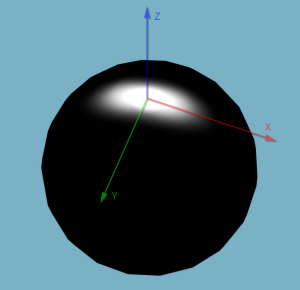

HLSL实现如下：

struct ASG
{
    float3 Amplitude;
    float3 BasisZ;
    float3 BasisX;
    float3 BasisY;
    float SharpnessX;
    float SharpnessY;
};
 
float3 EvaluateASG(in ASG asg, in float3 dir)
{
    float sTerm = saturate(dot(asg.BasisZ, dir));
    float lambdaTerm = asg.SharpnessX * dot(dir, asg.BasisX)
                                      * dot(dir, asg.BasisX);
    float muTerm = asg.SharpnessY * dot(dir, asg.BasisY)
                                  * dot(dir, asg.BasisY);
    return asg.Amplitude * sTerm* exp(-lambdaTerm - muTerm);
}

这篇各向异性球面高斯的论文还提供了两个公式，可用于提高球面高斯光源的镜面反射质量。第一个是新的扭曲算子，可以用NDF作为各向同性球面高斯，然后沿着视线方向拉伸产生比实际BRDF更好的各向异性球面高斯。另一个有用的公式是将各向异性球面高斯与各向同性球面高斯做卷积。可以用来将各向异性扭曲的NDF波瓣与球面高斯光源波瓣做卷积。下图左是球面扭曲，图中是各向异性扭曲，图右是实际的GGX分布。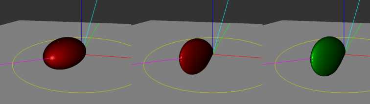

各向异性的分布看起来更接近实际的GGX NDF分布，因为有了之前缺少的垂直拉伸。下面是HLSL中的实现：

float3 ConvolveASG_SG(in ASG asg, in SG sg) {
    // The ASG paper specifes an isotropic SG as
    // exp(2 * nu * (dot(v, axis) - 1)),
    // so we must divide our SG sharpness by 2 in order
    // to get the nup parameter expected by the ASG formula
    float nu = sg.Sharpness * 0.5f;
 
    ASG convolveASG;
    convolveASG.BasisX = asg.BasisX;
    convolveASG.BasisY = asg.BasisY;
    convolveASG.BasisZ = asg.BasisZ;
 
    convolveASG.SharpnessX = (nu * asg.SharpnessX) /
                             (nu + asg.SharpnessX);
    convolveASG.SharpnessY = (nu * asg.SharpnessY) /
                             (nu + asg.SharpnessY);
 
    convolveASG.Amplitude = Pi / sqrt((nu + asg.SharpnessX) *
                                 (nu + asg.SharpnessY));
 
    float3 asgResult = EvaluateASG(convolveASG, sg.Axis);
    return asgResult * sg.Amplitude * asg.Amplitude;
}
 
ASG WarpDistributionASG(in SG ndf, in float3 view)
{
    ASG warp;
 
    // Generate any orthonormal basis with Z pointing in the
    // direction of the reflected view vector
    warp.BasisZ = reflect(-view, ndf.Axis);
    warp.BasisX = normalize(cross(ndf.Axis, warp.BasisZ));
    warp.BasisY = normalize(cross(warp.BasisZ, warp.BasisX));
 
    float dotDirO = max(dot(view, ndf.Axis), 0.0001f);
 
    // Second derivative of the sharpness with respect to how
    // far we are from basis Axis direction
    warp.SharpnessX = ndf.Sharpness / (8.0f * dotDirO * dotDirO);
    warp.SharpnessY = ndf.Sharpness / 8.0f;
 
    warp.Amplitude = ndf.Amplitude;
 
    return warp;
}
 
float3 SpecularTermASGWarp(in SG light, in float3 normal,
                           in float roughness, in float3 view,
                           in float3 specAlbedo)
{
    // Create an SG that approximates the NDF
    SG ndf = DistributionTermSG(normal, roughness);
 
    // Apply a warpring operation that will bring the SG from
    // the half-angle domain the the the lighting domain.
    ASG warpedNDF = WarpDistributionASG(ndf, view);
 
    // Convolve the NDF with the light
    float3 output = ConvolveASG_SG(warpedNDF, light);
 
    // Parameters needed for evaluating the visibility term
    float3 warpDir = warpedNDF.BasisZ;
    float m2 = roughness * roughness;
    float nDotL = saturate(dot(normal, warpDir));
    float nDotV = saturate(dot(normal, view));
    float3 h = normalize(warpDir + view);
 
    // Visibility term
    output *= GGX_V1(m2, nDotL) * GGX_V1(m2, nDotV);
 
    // Fresnel
    float powTerm = pow((1.0f - saturate(dot(warpDir, h))), 5);
    output *= specAlbedo + (1.0f - specAlbedo) * powTerm;
 
    // Cosine term
    output *= nDotL;
 
    return max(output, 0.0f);
}

使用各向异性扭曲后的高光效果看起来好了很多。